KMP Algorithm Why and How?

Notes

This blog is inspired by ICS161 which is a good source for understand and analysis KMP, and geeksforgeeks which provides concise and well explained code for C++, Python and Java.

There are different implemented versions of KMP, which may confuse you a lot, but you will understand all of them once you master KMP’s core idea.

Introduction

Knuth–Morris–Pratt algorithm which is also known as KMP algorithm, is an effective pattern search algorithm. It is used for solving the kind of problem: given a text string and a pattern string, determine whether the pattern appears somewhere in the text or not. In the following, we will give a force and naive solution for this problem, and then we speed it up by introduce the KMP solution.

Solution 1. Naive search

The naive solution is straight and easy to understand. It mainly consists of 2 loops, one outer loop indexed by $i$, one inner loop indexed by $j$. $i$ moves along the text str $s$, $j$ moves along the pattern str $p$.

def naive_search(s, p):
    # s: text, p: pattern
    ls, lp, ret = len(s), len(p), -1
    if lp == 0:
        ret = 0
    i, j = 0, 0
    while i < ls:
        j = 0
        while i + j < ls and j < lp and s[i + j] == p[j]:
            j = j + 1
        if j == lp:
            ret = i
            print("Find pattern in: {}".format(i))
        i = i + 1

Let’s look at a worst case first:

# a worst case: O(ls*lp)
s = "aaaaaaaaaaaaa...aaaaaaaaaaaaaaa"
p = "aaaab"
# illustration: x means mismatch at this position
    0123456789012...    
s[] aaaaaaaaaaaaa...aaaaaaaaaaaaaaa
i=0:aaaax
i=1: aaaax
i=2:  aaaax
...
i=ls:                             a  # meet text's end

Analysis of worst case $O(ls \times lp)$: we start from the 1st “a” in s, we need to compare $lp$ times till we know it is a mismatch, since the character “b” is at the end of the pattern str. But we are not sure that whether there exists a pattern in the following chars, to avoid skipping any matches, we start from 2nd “a” in s , and repeat the above search again, this time we still find out that it is a mismatch using $lp$ comparisions. Oops, we need to compare $ls lp$ times to know that there is no such pattern in the text. So the naive search* algorithm’s comparisions complexity is $O(ls \times lp)$.

Howerver, don’t be too frustrated. In practice you seldom meet the worst case. Under most circumstances, the mismatch doesn’t always happens at the end, so you will meet it earlier, thus you break the inner loop earlier. Well, the naive solution works not too bad in average.

Solution 2. KMP search: Skip redundant comparisions

The core idea of KMP is that we can skip non-essential comparisions in the naive search. So we need to figure out that which part of comparisions is essential and which part can be skipped. In fact, there are 2 parts can be skipped, one part is in the outer loop (skip some postions of $i$), the other is in the inner loop (skip some postions of $j$).

First part: skip some $i$s, the outer loop

In this section, we will show you why and how the outer loop can be skipped. First, let’s make a small pattern search challenge, and you can do it intuitively with the naked eye. (Forget about the algorithms!)

# case 1:
s = "ababaacbaabcdefab"
p = "abcdef"
# intuitive procedure
     01234567890123456    
s[]: abcdababcdecabcdef
i=0: abcdx
i=1:     abx
i=2:       abcdex
i=3:            x
i=4:             abcdef

Suppose the text $s$ is a fixed sequence, and the pattern is a box on trail, you can push it along the trail, but the text str is fixed there. In my intuitive procedure, you can see that from i=0 to i=1, I pushed my pattern box 4 steps at one time. I can do this because I know that pos 1, 2, 3 is “bcd” and no “a” exists there, so I omitted “bcd”. How did I know this information? Will this make a help?

The answer is “Yes”. It is the pattern who told me this info. Once you matched part of the pattern, you know what matched part is in the text str. This is the idea of KMP.

The above pattern is special without any repeated chars, let’s see another case with repeated chars.

# case 2:
s = "ababaaabaabaababab"
p = "aababaa"
# naive procedure
     01234567890123456    
T[]: aabaaababaabababa
i=0: aabax
i=1:    aax
i=2:     aababaa
i=3:          aababax
i=4:               ax
i=5:                x
i=6:                 a

Let’s look at i=0 and i=1 iters, after i=0, we only pushed ahead our pattern box 3 steps. We can’t push it directly to the mismatched pos 4, because we know that the already matched part after i=0 is “aaba”, if we pushed 4 steps, the 3rd “a” might be omitted, we just know the pos 4 is not “b”, but we don’t know whether it is an “a” or not. If we skip pos 3, we might lose a perfect match. To avoid this, we must be careful and only push 3 steps. It seems that, we the number of steps we can push depends on the pattern str’s structure. If there exists header-like substr inside the pattern’s body, we must be careful. If there doesn’t exist such header-like substrs, we can push our pattern box boldly. (what is “header-like”: e.g. for pattern: “aababaa”, the idx={1} (“a”), idx={3} (“a”) and idx={5,6} (“aa”) are all similar to header: “a” or “aa”, they are header-like substrs.)

Such header-like substrs are named as overlap or longest prefix suffix (lps) for short, that is, longest proper prefix which is also suffix. A proper prefix is prefix with whole string not allowed (can’t be equal to the origin str). For example, in str “aababaa”, the lps is “aa” (len = 2); in “aababa”, the lps is “a” (len = 1); in “aabab”, the lps is “” (len = 0). A lps table for “aababaa” are shown below, each lps[i] indicates the longest prefix suffix for str p[0…i] (i is included).

# lps table for pattern "aababaa"
p[] a a b a b a a
idx 0 1 2 3 4 5 6
lps 0 1 0 1 0 1 2

Given this table, you’ll know where to stop when you push your pattern box ahead. For example, assume that a mismatch occurs at pos $i$ of the text str and at pos $j$ of pattern str, our push should stop at the next header-like pos. Loot at the lps table, we find out that lps[$j - 1$] = $l$, which means the longest header-like substr of already matched part(note $j - 1$)’s length = $l$. Then we should push our box $j - l$ steps. So the next $i$’s pos is $i + (j - l)$.

How to generate the lps table will be explained below.

Second part: skip some $j$s, the inner loop

In this section, we will show you why and how the inner loop can be skipped. Again, we use case 2 as an example. For iter=0, it mismatched at pos 4, which means that s[0…3] are matched with pattern p[0…3], that is, s[0…3] = “aaba”. And for iter=1, since we already knew that s[3]=”a”, we don’t have to compare s[3] with p[0] again. We can start our comparation from p[1] instead of compare from p[0]. Note that, here we skipped some $j$. Similar to last section’s formulation, we can know where to start our $j$ when comparing patterns using lps table. It is easy to find out that, we start $j$ at the end of the header-like substr, that is, $j = l$.

# case 2:
s = "ababaaabaabaababab"
p = "aababaa"
# naive procedure
     01234567890123456    
T[]: aabaaababaabababa
i=0: aabax
i=1:    aax
i=2:     aababaa
i=3:          aababax
i=4:               ax
i=5:                x
i=6:                 a

Quick Review

Each time a mismatch occurs, we need to decide in the next iteration where $i$ should be and where $j$ should be. The computation of next $i$ and $j$’s positions is based on a pre-computed table lps table. The pseudo code of KMP algorithm is:

# input: text: s, pattern: p
compute the lps table of p;
i, j = 0, 0
while i is not at the end of s:
    match until a mismatch occurs or matched the whole pattern.
    if matched the whole pattern:
        print the start idx
    # we need to find out all matched patterns, so we continue
    update i
    update j

Compute lps table

In this section, we describe how to compute the lps table in detail.

# lps table for pattern "aababaa"
p[] a a b a b a a
idx 0 1 2 3 4 5 6
lps 0 1 0 1 0 1 2

To compute the above lps[j], suppose we knew lps[j - 1], we need to consider 2 situations:

If p[j] == p[lps[j - 1]] then the longest prefix suffix of p[0…j] enlongates by 1 (lps[j] = lps[j - 1] + 1).
If p[j] != p[lps[j - 1]], does it mean that longest prefix suffix of p[0…j] is “” and lps[j] = 0 ？

We explain situation 2 by 2 cases:

# situation 2.1:
p = "aabaacb"
p[] a a b a a c b
idx 0 1 2 3 4 5 6
lps 0 1 0 1 2 0 0
# situation 2.2:
p = "aabaaaa"
p[] a a b a a a a
idx 0 1 2 3 4 5 6
lps 0 1 0 1 2 2 2

In case 2.1, p[5] != p[lps[4]] (“c” != “b”), lps[5] is 0. Wheras in case 2.2, p[5] != p[lps[4]] (“a” != “b”), lps[5] is 2. So what’s the difference between the 2 subsituations?

If you’re carefully enough, you’ll find out that: in situation 2.1, p[3,4] = “aa” is header-like, p[4,5] = “ac” is not because it contains “c”, which is not in the header. In situation 2.2, p[3,4] = “aa” is header-like, p[4,5] = “aa” is also header-like. So we need to fingure out whether the current p[j] can enlongate part of the previous lps and construct a new header-like substr. If it does, lps[j] is the new substr’s length, if doesn’t, we need to repeat the procedure till the green part is “”, cur_len = 0.

def compute_lps_table(p):
    # input: p
    lp = len(p)
    lps = [0] * lp
    i, cur_len = 1, 0  # cur_len is current longest prefix suffix length
    while i < lp:
        if p[i] == p[cur_len]:  # situation 1: p[j] == p[lps[j - 1]]
            cur_len += 1
            lps[i] = cur_len
            i += 1
        else:  # situation 2: p[j] != p[lps[j - 1]]
            if cur_len > 0: # situation 2.1
                cur_len = lps[cur_len - 1]
            else:  # situation 2.2
                lps[i] = 0
                i += 1
    return lps

In the above code, line # case 4 is a bit hard to understand. Now, we analysis this line of code in detail. The figure below explain what we want to do. 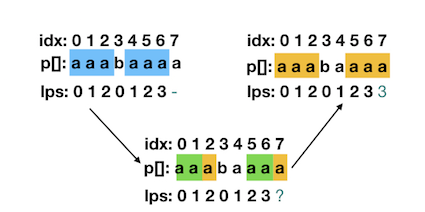lps explaination

The blue part is what we knew: cur_len = lps[j-1] = 3, the orange part is what we want to find. If we want to find the orange part, we need to figure out the length of the green part. Here is the derivation process, based on transitivity equation:

# Proof
∵ len(p[0,1,2]) == len(p[4,5,6]) = cur_len
∴ len(p[1,2]) == len(p[5,6])
∵ len(p[0,1]) == len(p[1,2]) = lps[cur_len - 1]
∴ len(p[5,6]) = len(p[0,1]) = lps[cur_len - 1]

So that we find the length of green part p[5,6]: lps[cur_len - 1]。 Once the green part is founded, we can judge that: if the green part + p[j] can be a lps, then lps[j] = len(green part) + 1, else we repeat the previous steps till we can make a decision (belongs to situation 1 or situation 2.1). It’s a recursive procedure, so we use cur_len to save the green part’s length.

KMP Algorithm

In this section, we implement KMP algorithm in Python. Below is the code, explaination is thorough.

def kmp_search(s, p, lps):
    # input: text:s, pattern:p, lps table: tbl
    # idx = -1 if not found
    i, j, ls, lp, idx = 0, 0, len(s), len(p), -1
    while i < ls:
        # match till a mismatch occurs or match whole pattern
        while i + j < ls and j < lp and s[i + j] == p[j]:
            j = j + 1
        # perfect match!
        if j == lp:  
            idx = i
            print("Found pattern at: {}".format(idx))
        # update i
        i = i + max(1, j - lps[j - 1])# update j
        # update j
        # when j != 0, note that in python lps[-1] means the last element in lps
        # when j == 0: a mismatch occurs at the first character, j should keep its value: 0
        if j != 0:
            j = lps[j - 1]
    return idx

Postscript

KMP algorithm is a classic pattern searching algorithm, hope this article will help you understand it better. I spent several days to figure this out, so if you meet some knots, you may need to think it over and over till you fully master it. After that, you can compare its idea with other pattern search algorithms, you’ll find that they are all interesting.

If you find any issue, please contact me through the email.