Tensorflow Get Started

这篇博客的主要内容来自于Tensorflow的英文官方教程：
Getting started with tensorflow!，同时加入了个人的理解和知识点的扩充。
感谢上面那篇文章的作者，很棒的入门的教程！

Tensorflow——An open-source software library for Machine Intelligence
–致力于深度学习的Python开源库。

• Lowlevel API：较为底层的API，适合高级使用者:比较care模型性能的研究人员，和对底层代码很感兴趣的人员。
• Highlevel API: 高层一点的API，较lowlevel API好学，易用。能够帮助你方便地管理datasets，模型，完成训练和预测的工作。
• 请注意那些名字里有contrib的API: 这些API仍在developing阶段，tensorflow的代码是开源的，这意味着那些API可能处于变化中。如果感兴趣，你也可以加入到tensorflow的coding队伍中，变成一个为其他开发人员设计工具的开发人员。

我的寄语：
Dear friend,
建议你在学习tensorflow之前，

• 丰富自己的想象力， 因为你的脑海中需要构建出一幅data flow graph，这幅图能让你的代码思路更加清晰，这很重要，尤其是当你的模型越来越复杂，需要使用的tensorflow功能越来越多时。
• 不要着急去看Github上别人写的代码，先花些时间弄懂tensorflow 设计的抽象概念，这在之后能够帮助你快速理解别人的代码，并且自己也能够写出更棒的代码！
• Tensorflow官网的documents很多，如果你是一个完完全全的新手，建议你从Getting Started With TensorFlow开始学习。
• 学习资料比较长，请多一点耐心读完，并且随时动手敲代码！

1. 必须理解的概念：

1. Tensors: (数据)
   任意维数的array，tensor的rank指的是array的维度:
   eg.

   1 2 3 4 5

   # tensor examples 3 # rank:0, 1-d array, shape:[] [1.,2.,3.] # rank:1, 1-d array, shape:[3] [[1.,2.,3.], [2.,1.,3.]] # rank:2, 2-d array or matrix, shape:[2, 3] [[[1.,2.,3.], [2.,1.,3.]]] # rank:3, 3-d array or matrix, shape:[1, 2, 3]

   tensorflow把封装成一个Python类，使用类中的方法，可以方便地对array进行管理和操作。

2. Computational Graph: (计算图)
   数据量越大，计算过程越复杂，越需要一个清晰的思路整理数据处理的流程。Tensorflow通过data flow graph来记录对每部分数据要分别进行什么操作。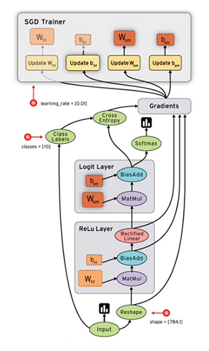
   
   Tensorflow把对数据的操作化作directed graph中的节点，数据（tensor）就是节点直接相连的边，可以想象数据在图上有向地流动，每次流进节点就会进行某种指定的操作，然后流出的是操作之后的数据。Tensorflow这个名字很明确地表达了自己的本质呢。
   简单说来，tensorflow做的事情主要分为两步：

   1. 生成computational graph;

   2. 执行computational graph;

      Computational graph的node，接受0个或任意多个tensor作为input，然后output一个tensor作为输出。是的，node可以没有输入，例如node本身就是一个constant，它不接受任何输入，执行的动作是：把存储在自己内部的数值输出。下面我们创建两个constant node试试看：

      1 2 3 4 5 6 7 8 9 10

      const_node_1 = tf.constant(3.0, tf.float32) const_node_2 = tf.constant(4.0) # float默认就是tf.float32，可以不必显式指明 const_node_3 = tf.constant(5) # int 类型 # output >>> const_node_1 <tf.Tensor 'Const_11:0' shape=() dtype=float32> >>> const_node_2 <tf.Tensor 'Const_10:0' shape=() dtype=float32> >>> const_node_3 <tf.Tensor 'Const_9:0' shape=() dtype=int32>

Â
这里并没有显示每个constant内部存储的值，但是别担心，在它们真正参与计算时，3.0,4.0和5都会乖乖出现的。这里我们只是生成了一个包含三个constant nodes的computational graph，它现在是静态的，并没有进行任何实质上的操作，下一步我们通过run这个graph，让数据真正地flow起来!

1. Session：(会话)
   Computational graph的运行必需要处在一个叫做：session的环境中才可以进行，session像一个厉害的大管家，为我们隔离了许多复杂的控制和状态，让我们不必为这些琐碎的问题操心。下面我们就来创建一个session，期待看到数据流动起来的样子：

   1 2 3 4 5

   >>> sess = tf.Session() >>> sess <tensorflow.python.client.session.Session object at 0x7f5fddfaab38> >>> sess.run([const_node_1, const_node_2]) [3.0, 4.0] # 3.0 and 4.0 as we expected

   来点更复杂一些的操作：比如让上面两个节点的值相加：3.0 + 4.0

   1 2 3 4

   add_node_1 = tf.add(const_node_1, const_node_2) print(sess.run(add_node_1)) # output 7.0

2. Placeholder: (data)
   可能你还是觉得太简单了，两个常数相加挺无聊的，我想自己指定两个加数的值：

   1 2 3 4 5 6 7 8

   >>> a = tf.placeholder(tf.float32) >>> b = tf.placeholder(tf.float32) >>> add_node_2 = tf.add(a, b) # 等价于：add_node_2 = a + b # output >>> sess.run(add_node_2, {a:1, b:5})# 虽然是int, 仍然当成tf.float32 6.0 >>> sess.run(add_node_2, {a:[1,3], b:[2.2,3.4]}) [ 3.20000005 6.4000001 ]

   这里我们用到了Placeholder：它相当于函数在定义时的形参，在使用的时候就会被赋予具体的值；同时我们可以指定传入参数的类型：例如 tf.float32。Placeholder 在定义时不能初始化，它的赋值必须在run时进行。
   注：观察到上面1 + 2.2 和3+3.4的结果比真实值稍稍大了一点点，通过尝试tf.float16, tf.float64的 placeholder(), 可以发现，小数的精度越高这个误差越小。
   下面我们更进一步实现(a + b) * c 的计算过程：

   1 2 3 4 5 6 7 8 9 10 11

   # 使用两个node实现 >>> c = tf.placeholder(tf.float32) >>> add_mult_node_1 = add_node_2 * c # output >>> sess.run(add_mult_node_1, {a:1.1, b:2.2, c:3.}) 9.9 # 使用一个node实现 >>> add_mult_node_2 = (a + b) * c # output >>> sess.run(add_mult_node_2, {a:1.1, b:2.2, c:3.}) 9.9

   在这个过程中，我们需要在心里绘制出一幅computational graph， 如果操作很多也可以直接画在纸上。
   Important: Placeholder如果在定义时被赋值，将会报错! Its value must be fed using the feed_dict optional argument to Session.run(), Tensor.eval(), or Operation.run().

3. Variables：(params)
   在Tensorflow中，我们使用Variables来存储和更新parameters。 Variables 是存储在内存中的 tensors. 它们必须在launch graph之前显式初始化，还可以training过程中和training结束之后存储到你的磁盘上，以便下次直接使用该模型。

   我们需要明确Placeholder和Variable的使用：

   • Input data 通常声明为Placeholder
   • Model 的参数通常声明为Variable
   • Placeholder 为feed data而生，定义时不能赋值，其内容为空，执行时通过 run()，eval() 等方法赋予实际值

   • Variable 为模型参数而生，定义时必须提供初值，数据类型可以是任意type、shape 的 Tensor 。

     下面我们通过一个简单的Linear Model看看如何使用Variable定义模型参数：lm = W * x + b

     1 2 3 4

     W = tf.Variable([.3], tf.float32) b = tf.Variable([-.3], tf.float32) x = tf.placeholder(tf.float32) linear_model = W * x + b

     初始化Variables:

     1 2	init = tf.global_variables_initializer() sess.run(init)

     run init会初始化整个graph中的所有全局Variables；TensorFlow是lazy执行的，在run之前，所有的Variables都没有被赋予实际的值。
     下一步我们feed一组input样本x给我们可爱的linear model，看它会有什么输出：

     1 2 3

     print(sess.run(linear_model, {x:[1,2,3,4]})) # output [ 0. 0.30000001 0.60000002 0.90000004]

     现在我们需要知道这个linear_model的预测效果如何，接下来我们将给出样本的真实值y, 通过_lossfunction对比模型的输出_ym和真实值y之间的差异。loss function的类型很多，这里选择简单的平方误差函数：loss = (y_m - y)^2

     1 2 3 4 5 6

     y = tf.placeholder(tf.float32) squared_deltas = tf.square(linear_model - y) # 单个样本预测误差 loss = tf.reduce_sum(squared_deltas) # 整体样本预测误差 print(sess.run(loss, {x: [1,2,3,4], y: [0,-1,-2,-3]})) # output 23.66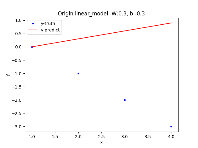

     
     哎呀，这个模型的误差足足有23.66，效果不够理想！我们需要对它进行改进，通常训练模型的过程会通过最小化误差函数自动调整模型参数，从而使模型达到最优，这里我们为了方便，就直接给出最优模型。best_linear_model = -1.0 * x + 1.0， 这一步我们更新模型参数W,b的值为-1.0， 1.0。
     更新Variable的值，可以通过tf.assign()方法实现：

     1 2 3 4 5 6 7 8

     # assign best val for W and b fix_W = tf.assign(W, [-1.]) fix_b = tf.assign(b, [1.]) # do the operation acturally sess.run([fix_W, fix_b]) print(sess.run(loss, {x: [1,2,3,4], y: [0,-1,-2,-3]})) # output 0.0

     现在model的loss是0，效果有了很大的提升！

4. 自动调参：
   既然是machine learning，不能每次都手动更新参数吧，别着急，这一步我们学习如何自动更新模型参数，从而提升预测效果。
   Tensorflow提供了许多类型的optimizer，在train阶段，这些optimizer能够自动优化你指定的目标函数，通常是让损失函数达到最小。tf.train.GradientDescentOptimizer是最简单的optimizer。
   其原理是：梯度下降法。把要优化的目标函数想象成一座座连绵的山，我们从山中的任意一点开始下山，目标是尽快到达山下的最低点，梯度下降法的策略是：求当前位置的梯度g（最陡的方向下山最快），然后沿着梯度的负方向走一步，这一步应该迈的距离是learningrate，也叫步长_。步长的太大可能会导致错过最低点，太小又可能导致收敛的太慢，因此需要小心地选择一个合适的步长。
   备注: GradientDescent算法不能保证每次都收敛到全局最优解，有时候你很可能得到的只是一个局部最优解。
   当然，optimizer使用起来十分easy，因为它就是个黑盒子，我们只需要告诉它要优化的目标函数，它就会自动帮我们找到最优解。

   1 2 3 4 5 6 7 8 9 10 11 12 13

   # choose an optimizer optimizer = tf.train.GradientDescentOptimizer(0.01) # tell it what to do next train = optimizer.minimize(loss) # init W, b with sess.run(init) # train loop for i in range(1000): sess.run(train, {x:[1,2,3,4], y:[0,-1,-2,-3]}) print(sess.run([W, b])) # output [array([-0.9999969], dtype=float32), array([ 0.99999082], dtype=float32)]

   经过1000次迭代之后，W,b 已经十分接近标准答案-1.0,1.0了，我们完成了就是自动学习参数的过程！

2. 完整的模型训练过程：

上一步我们直接给出了模型的最优参数，接下来我们进行一次真正意义上的Machine Learning，让模型自己学习出最优的W,b。

1
2
3
4
5
6
7
8
9
10
11
12
13
14
15
16
17
18
19
20
21
22
23
24
25
26
27
28
29
30
31
32
33
34
35
36
37
38
39
40
41
42
43
44
45
46
47
48
49
50
51
52
53
54
55
56
57
58
59
60
61
62
63
64
65
66
67
68
69
70
71
72
73
74
75
76
77
78
79
80
81
82
83

#!/usr/bin/python
# -*-coding:utf-8-*-
"""complete_example_tf.py
Description: a complete example for tensorflow tutorial.
Date: 2017-05-19
Author: MonkandMonkey
"""
import numpy as np
import tensorflow as tf
import matplotlib.pyplot as plt
# ============================
# A complete tensorflow example
# ============================
def complete_try():
    # max iteration times
    max_iter = 1000
    '''Construct the computational graph'''
    # model parameters
    W = tf.Variable([.3], tf.float32)
    b = tf.Variable([-.3], tf.float32)
    # model input and output
    x = tf.placeholder(tf.float32)
    liner_model = W * x + b  # predict y
    y = tf.placeholder(tf.float32)  # true y
    # define loss function
    suqared_deltas = tf.square(liner_model - y)
    loss = tf.reduce_sum(suqared_deltas)
    # choose an optimizer
    optimizer = tf.train.GradientDescentOptimizer(learning_rate=0.01)
    # set the train object
    train = optimizer.minimize(loss)
    '''Prepare training data'''
    x_train = [1, 2, 3, 4]
    y_train = [0, -1, -2, - 3]
    '''Run the graph'''
    sess = tf.Session()
    init = tf.global_variables_initializer()
    sess.run(init)  # initialize params: W, b
    # training loop
    for i in range(max_iter):
        if i % 50 == 0:
            curr_W, curr_b, curr_loss = sess.run([W, b, loss], feed_dict={x: x_train, y: y_train})
            print("[{:0>3}] - W: {:<5.4f}, b: {:<6.4f}, loss: {:<6.4f}".format(i, curr_W[0], curr_b[0], curr_loss))
        sess.run(train, feed_dict={x: x_train, y: y_train})
    # evaluate the accuracy
    trained_W, trained_b, trained_loss = sess.run([W, b, loss], feed_dict={x: x_train, y: y_train})
    print("Training result:")
    print("  W: {:<5.4f}, b: {:<6.4f}, loss: {:<6.4f}".format(trained_W[0], trained_b[0], trained_loss))
    return trained_W[0], trained_b[0]
# ============================
# Pic for tensorflow tutorial
# ============================
def pic_tensorflow(W, b):
    y = np.array([0, -1, -2, -3])
    x = np.array([1, 2, 3, 4])
    y_m = W * x + b
    plt.plot(x, y, 'b.', x, y_m, 'r-')
    # add labels
    plt.xlabel("x")
    plt.ylabel("y")
    # add legends
    plt.legend(["y-truth", "y-predict"])
    # add title
    plt.title("Best linear_model: W={:.2f}, b={:.2f}".format(W, b))
    plt.show()
    print("Plot pic_tensorflow: a simple plot for tensorflow get started!")
if __name__ == '__main__':
    print("Start running!")
    W, b = complete_try()# train the model
    pic_tensorflow(W, b) # plot the model

这里借用tensroflow的computational graph: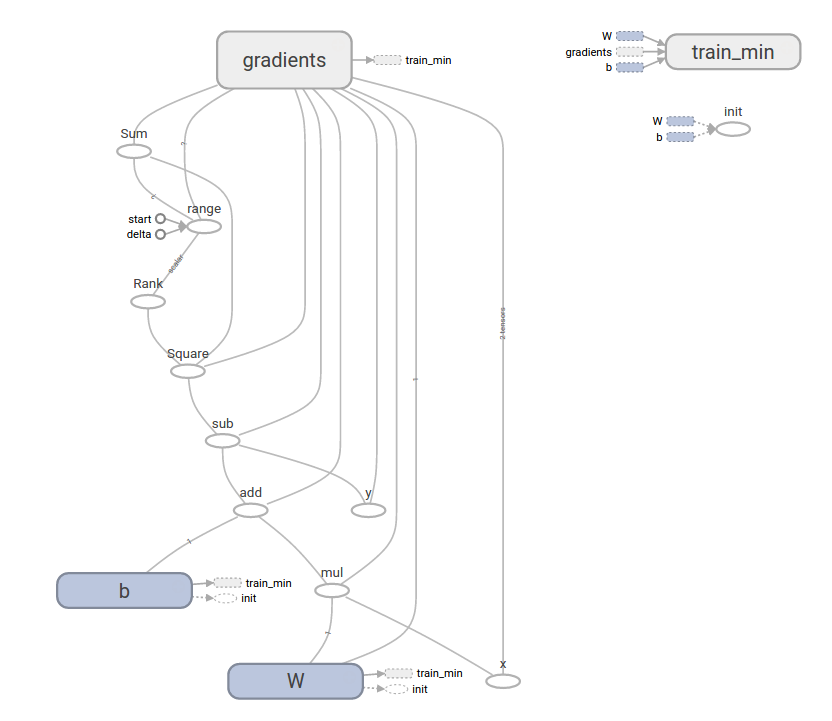

这幅图远比我们想象得要复杂一些，不过很多细节都是tensorflow帮我们补充上的，我们只需要确保那些关键细节正确。

3. 还能更简单？

tf.contrib.learn 让 Machine learning 的过程进一步地简化，属于更加high level的API，让整个machine learning的过程看起来越来越像你草稿纸上的几行简单的“算法思路”。
仍以Linear Model为例，我们看看使用tf.contrib.learn如何完成相同的事情：

1
2
3
4
5
6
7
8
9
10
11
12
13
14
15
16
17
18
19
20
21
22
23

import tensorflow as tf
# NumPy 包通常用于处理数据
import numpy as np
# input data：only 1 feature - x
features = [tf.contrib.layers.real_valued_column("x", dimension=1)]
# estimator: provide the handler for model's fitting and evaluation
# 更多类型的estimator可以查阅API
estimator = tf.contrib.learn.LinearRegressor(feature_columns=features)
# read and set up data sets.
# numpy_input_fn: 读入、划分数据集为一个个batch
# 1 epoch: 使用一遍data set
x = np.array([1., 2., 3., 4.])
y = np.array([0., -1., -2., -3.])
input_fn = tf.contrib.learn.io.numpy_input_fn({"x": x}, y, batch_size=4,
                                                  num_epochs=1000)
# 训练迭代1000次
estimator.fit(input_fn=input_fn, steps=1000)
# 检验模型的效果（实际使用应当在test set进行）
print(estimator.evaluate(input_fn=input_fn))

tf.contrib提供了许多常用的model,例如：linear regression,logistic regression, linear classification, logistic classification, and many neural network classifiers and regressors。当然，如果你想自己定制model,也是可以的，下面就是一个自己定制的Linear Model例子：

1
2
3
4
5
6
7
8
9
10
11
12
13
14
15
16
17
18
19
20
21
22
23
24
25
26
27
28
29
30
31

# featiures: [x], labels: true y, mode:
def model(features, labels, mode):
    # Build a linear model and predict values
    W = tf.get_variable("W", [1], dtype=tf.float64)
    b = tf.get_variable("b", [1], dtype=tf.float64)
    y = W * features['x'] + b
    # Loss sub-graph
    loss = tf.reduce_sum(tf.square(y - labels))
    # Training sub-graph
    global_step = tf.train.get_global_step()
    optimizer = tf.train.GradientDescentOptimizer(0.01)
    train = tf.group(optimizer.minimize(loss),
                     tf.assign_add(global_step, 1))
    # ModelFnOps connects subgraphs we built to the
    # appropriate functionality.
    return tf.contrib.learn.ModelFnOps(
        mode=mode, predictions=y,
        loss=loss,
        train_op=train)
if __name__ == '__main__':
    estimator = tf.contrib.learn.Estimator(model_fn=model)
    # define our data set
    x = np.array([1., 2., 3., 4.])
    y = np.array([0., -1., -2., -3.])
    input_fn = tf.contrib.learn.io.numpy_input_fn({"x": x}, y, 4, num_epochs=1000)
    # train
    estimator.fit(input_fn=input_fn, steps=1000)
    # evaluate our model
    print(estimator.evaluate(input_fn=input_fn, steps=10))

上一部分中的tf.contrib.learn.LinearRegressor，是tf.contrib.learn.Estimator的一个sub-class, 如果我们要定义自己的model, 也需要继承Estimator类。可以通过定义model_fn函数，来描述是一个怎样的model。model_fn中需要指明:fit, loss, evaluate，整个流程看起来非常像我们第二部分中使用low level API实现的例子： 定义parameters, 定义model， 定义loss, optimizer。就好像我们分别设计个几个sub-graphs，然后使用ModelFnOps把各个子图连接起来。

读到这里，你应该已经了解了tensorflow的基本套路，面对长长的示例代码也不怕了, 写起代码来也更得心应手。
希望本文对你的理解有所帮助！(^_^)